Import bibench like any Python module:
>>> import bibench
If the import fails, make sure that BiBench is on your PYTHONPATH.
BiBench contains many submodules, but to save time you can use the bibench.all module, which imports the most useful functions into one place:
>>> import bibench.all as bb
First we need a dataset on which to run our biclustering algorithms. BiBench can generate synthetic data for testing purposes. Here we make a dataset with upregulated biclusters:
>>> data, expected = bb.make_const_data(bicluster_signals=[5,5,5], shuffle=True)
The list of hidden biclusters, expected, will be useful later to see how well an algorithm has done. The dataset is a standard numpy.ndarray, so we can do all the usual things like examine its shape:
>>> data.shape
(300, 50)
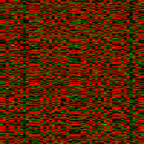
BiBench supports visualizing data and biclusters in various ways. We can also view a heatmap of the data:
>>> bb.heatmap(data)
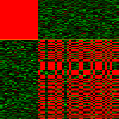
We can also sort the dataset so that the first expected bicluster is contiguous:
>>> bb.heatmap(data, expected[0], local=False)
Now we want to cluster the dataset using BiMax. But BiMax requires that the data be binarized. We use QUBIC’s method of discretization to make this dataset binary:
>>> bin_data = bb.qubic_binarize_up(data)
Now we can cluster the dataset and see how well BiMax did:
>>> found = bb.bimax(bin_data)
>>> bb.jaccard_list(expected, found)
ListScore(relevance=0.055462621590093929, recovery=1.0)
It looks like BiMax found all the biclusters, but also found lots of extra ones that are hurting its relevance score. The filter function is useful in this case; here filter out small biclusters:
>>> filtered = bb.filter(found, minrows=5, mincols=5)
>>> bb.jaccard_list(expected, filtered)
ListScore(relevance=1.0, recovery=1.0)
Note that filter also removes duplicate biclusters.
Now let’s try clustering a real microarray dataset. If rpy2, R, and Bioconductor are installed, we have access to all of the functionality of Bioconductor, including lots of datasets. A list of all experiment data packages is available here. (It is also possible to get a list interactively. See rpy2’s documentation for interactive work)
Let’s install the ALL data, which consists of 128 microarrays from patients with acute lymphoblastic leukemia (ALL). We first need to get the bioclite command, which requires an internet connection:
>>> bioclite = bibench.rutil.get_bioclite()
>>> bioclite('ALL')
Now that the data is installed, we can get it:
>>> data = bb.get_bioc_data('ALL')
Gene expression data files have labelled rows (genes/probes) and columns (samples). We can access them as members of our data. Here we have Affymetrix probes for our row labels:
>>> data.genes[0:3]
['1000_at', '1001_at', '1002_f_at']

>>> data.samples[0:3]
['01005', '01010', '03002']
This time we use QUBIC for clustering:
>>> found = bb.qubic(data)
Since this is a real dataset, the true biclusters are unknown. However, we can do Gene Ontology enrichment analysis on each bicluster. Since this dataset was obtained from Bioconductor, we can find which annotation package to use by simply examing the annotation attribute:
>>> data.annotation
'hgu95av2'
We check the biclusters for enriched Gene Ontology terms, using the datasets probes as the gene universe:
>>> enriched = [bb.enrichment(f, data.annotation, data.genes) for f in found]
>>> enriched[0]
It is easy to get a GO id’s full annotation. For instance, suppose we wanted to get GO:0048870‘s full annotation:
>>> bb.goid_annot('GO:0048870')
GoAnnot(goid='GO:0048870',
        term='cell motility',
        ontology='BP',
        synonym=None,
        secondary=None,
        definition='Any process involved in the controlled self-propelled movement of a cell that results in translocation of the cell from one place to another.')
Then using bb.goid_annot we can get the first bicluster’s actual enriched terms:
>>> [annot.term for annot in [bb.goid_annot(e.goid) for e in enriched[0]]]
['cardiovascular system development',
 'blood vessel development',
 'extracellular matrix organization',
 'muscle tissue development',
 'cell adhesion',
 'collagen fibril organization',
 'muscle organ development',
 'cell motility',
 'muscle contraction',
 'angiogenesis']
Finally, we export the first six biclusters in the BicOverlapper format, to allow visualization using the BicOverlapper visualization tool:
>>> bb.write_bicoverlapper([found[0:6]], './all-data-qubic-biclusters.txt', data.genes, data.samples)
After importing the result and choosing the Overlapper view, this is the result:
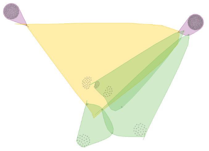
Clearly these biclusters do not overlap much.
The Gene Expression Omnibus is a handy resource for expression data. BiBench provides an interface to the geometadb package, so we can query GEO metadata to find the appropriate dataset. The first time this functionality is used, the SQLlite database is automatically downloaded and stored in $HOME/.bibench/GEOmetadb.sqlite.
Suppose we want to find a curated (GDS) dataset that was generated from an Affymetrix chip:
>>> bb.geo_query("select gds from gds join gpl on gds.gpl=gds.gpl where gpl.manufacturer='Affymetrix'")
>>> len(result[0])
2721
There are 2721 such GDS datasets. The result of our query is an rpy2.robjects.vectors.DataFrame, with one column for each argument to select:
>>> type(result)
rpy2.robjects.vectors.DataFrame
We examine the first five datasets:
>>> result[0][0:5]
<StrVector - Python:0x188f4bcc / R:0x13ce5458>
['GDS5', 'GDS6', 'GDS10', 'GDS12', 'GDS15']
BiBench can automatically download and import GDS datasets. Here we get GDS3715:
>>> data = bb.get_gds_data(3715)
The dataset is cached in $HOME/.bibench/gds, so future calls to bb.get_gds_data(3715) will not download the whole dataset again.
Cluster the dataset using CPB:
>>> found = bb.cpb(data, 10)
BiBench automatically maps a GDS dataset’s GPL platform to the appropriate Bioconducter annotation database, if possible. Let’s make sure it worked:
>>> data.annotation
'hgu95av2'
It did indeed work. So it is easy to perform a Gene Ontology enrichment analysis:
>>> enriched = [bb.enrichment(f, data.annotation, data.genes) for f in found]